Quickstart
Description
Fit a CALM on a synthetic problem with one known interaction, read the
model card, see where it stands between a GAM and the black box it
learns from, read why it split what it split, plot the fitted curves and
take one prediction apart. The code is
examples/01_quickstart.py.
Reading time
Approx. 5' to read.
A problem with one interaction
Three features, uniform in [-1, 1]. The effect of x3 depends on the sign
of x2: a sine when x2 >= 0, a cosine when x2 < 0.
import numpy as np
import pandas as pd
from sklearn.model_selection import train_test_split

rng = np.random.default_rng(0)
X = pd.DataFrame(rng.uniform(-1, 1, (3000, 3)), columns=["x1", "x2", "x3"])
y = (
    X["x1"] ** 2
    + np.log(np.abs(X["x2"]))
    + 2 * np.where(X["x2"] >= 0, np.sin(np.pi / 2 * X["x3"]), np.cos(np.pi / 2 * X["x3"]))
    + rng.normal(0, 0.3, len(X))
)
X_train, X_test, y_train, y_test = train_test_split(X, y, test_size=0.2, random_state=0)
A GAM gives x3 one curve, so it has to average the sine and the cosine.
One call fits everything
from calm_additive import CALMRegressor

calm = CALMRegressor(max_partition_depth=1)
calm.fit(X_train, y_train)
fit trains a black box (XGBoost by default), looks for regions where a
feature's effect differs, keeps the regions that matter, and fits one curve
per (feature, region). max_partition_depth=1 allows each feature at most two curves.
👉 A DataFrame brings its column names along; a numpy array works too, with
features named x_0, x_1, ....
The model on one screen
calm.print_summary(X_test, y_test)
  ════════════════════════════════════════════════════════════════════════
  CALM regressor  ·  target: y
  ════════════════════════════════════════════════════════════════════════

  MODEL
  ────────────────────────────────────────────────────────────────────────
    trained on    2,400 rows · 3 features
    structure     4 curves · 1 partition · 1 conditional interaction
    baseline      −0.034  (the average prediction)

  WHERE IT STANDS                            on the data passed · 600 rows
  ────────────────────────────────────────────────────────────────────────
                                                          RMSE          R²
    GAM         ebm curves, no partitions                0.885       0.717
    CALM                                                 0.372       0.950
    black box   the teacher (xgb)                        0.411       0.939

    CALM is above the black box in R²

  FEATURES                          importance = mean |contribution|, in y
  ────────────────────────────────────────────────────────────────────────
    feature       importance                curves  depends on
    ──────────────────────────────────────────────────────────────────────
    x3                  1.07  ████████████       2  x2
    x2                  0.73  ████████           1  —
    x1                  0.25  ███                1  —

  PARTITIONS                                            one curve per leaf
  ────────────────────────────────────────────────────────────────────────
    x3
    ├─ x2 < 0.00   n = 1,244
    └─ x2 ≥ 0.00   n = 1,156
print_summary() prints the model card: how large the model is, each feature's
importance and what its curves depend on, and every partition as a tree.
x3 has two curves, one per side of x2 = 0: the interaction that was put
in the data.
CALM closes the gap to the black box
Because held-out data was passed, the card also says where it stands. The
GAM is the same curve fitter with no partitions, so the only difference
between the first two rows is the two curves of x3. Here CALM even ends
above its teacher.
The ledger says why
calm.chain_.show()
  EXPLAINED VARIANCE
  ────────────────────────────────────────────────────────────────────────
    step         split on                 solo     ΔR²      R²       heter
    ──────────────────────────────────────────────────────────────────────
    GAM          (all features global)       —       —   75.2%           —
  + x3           x2                     +20.6%  +20.6%   95.8% 0.76 → 0.15
    ──────────────────────────────────────────────────────────────────────
    FINAL                                                95.8%

  REJECTED SPLITS                                            min gain 1.0%
  ────────────────────────────────────────────────────────────────────────
    feature      split on                 solo     ΔR²    reason
    ──────────────────────────────────────────────────────────────────────
  ✗ x2           x3                     +16.0%  -15.3%    redundant

    ✗ redundant: it would explain variance on its own (see solo),
      but the accepted splits already account for it.
One split was kept: x3, conditioned on x2. It lifts the additive
surrogate from 75.2% to 95.8%. The mirror split, x2 conditioned on x3,
describes the same interaction a second time, so it was rejected as
redundant.
The R² in the ledger is not test accuracy
It measures how much of the black box an additive model explains, on the training data. Test accuracy is the where it stands block above.
The model is its plots
calm.plot_curves()
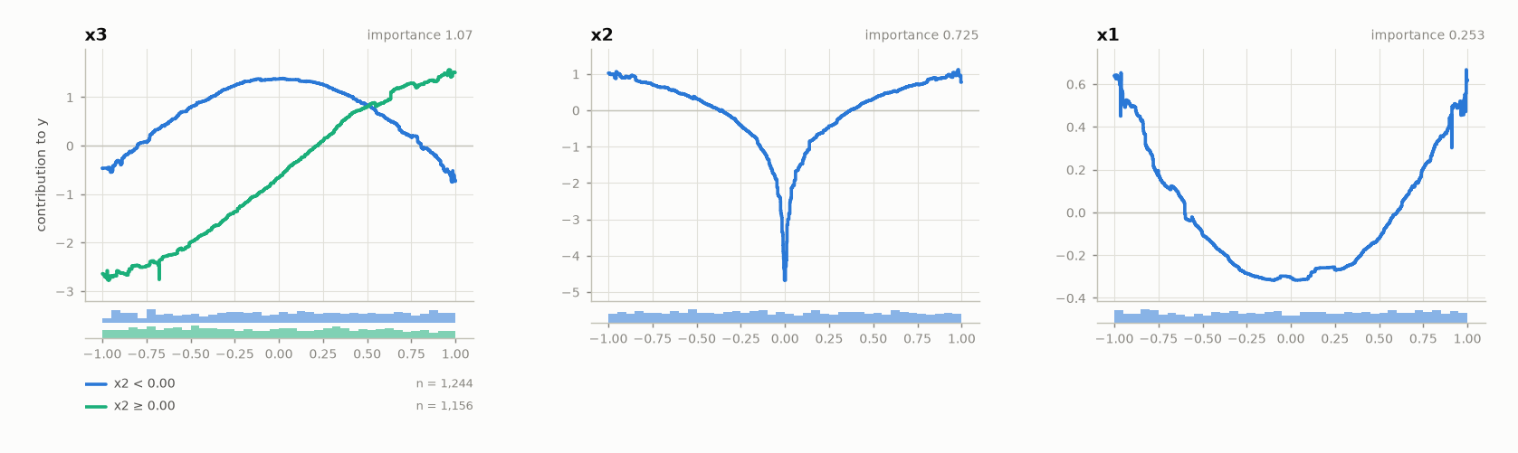
x3 has two curves: the cosine when x2 < 0, the sine when x2 >= 0. The
strip under each panel shows where the training rows are, one row of bars
per region. A prediction is the baseline plus one value read off each panel;
for x3, off the curve whose condition the row satisfies.
👉 calm.plot_curves("x3") draws one feature large, calm.plot_importance() the
features by importance.
One prediction, taken apart
row = X_test.iloc[0]
calm.print_prediction(row)
  PREDICTION                                                     y = −3.26
  ────────────────────────────────────────────────────────────────────────
    feature = value     because               contribution
    ──────────────────────────────────────────────────────────────────────
    x3 = -0.9732        x2 ≥ 0.00                    −2.71 ███████│
    x1 = -0.1198                                     −0.31       █│
    x2 = 0.3129                                      −0.20       █│
    ──────────────────────────────────────────────────────────────────────
    baseline (average prediction)                    −0.03
    + contributions                                  −3.22
    = y                                              −3.26
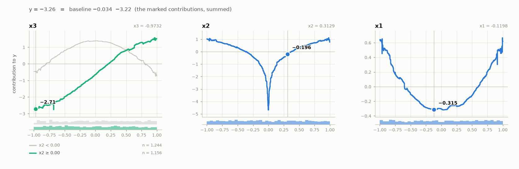
The lines add up to the prediction exactly. x3's line names the region
whose curve was read. The same row on the curves:
calm.plot_curves(at=row)
👉 calm.plot_prediction(row) draws the ledger as a waterfall;
calm.contributions(X) returns the numbers for many rows at once.
Where to next
- A real dataset: the same steps on Bike Sharing
- How it works: what
fitdoes, step by step - Choosing the knobs:
max_partition_depth,min_r2_gainand the rest