A real dataset
Description
CALM on Bike Sharing: hourly bike rentals, 17,379 rows, 12 features, some
of them categorical. The code is
examples/02_real_data.py, which also runs on
California Housing, Phoneme, or your own CSV.
Reading time
Approx. 5' to read.
A DataFrame goes straight in
from sklearn.datasets import fetch_openml
from sklearn.model_selection import train_test_split

df = fetch_openml("Bike_Sharing_Demand", version=2, as_frame=True).frame
X, y = df.drop(columns="count"), df["count"].astype(float)
X_train, X_test, y_train, y_test = train_test_split(X, y, test_size=0.2, random_state=0)
season, holiday, workingday and weather are pandas categoricals.
CALM encodes them itself and keeps their level names for the rules and the
plots. y is a pandas Series, so its name, count, becomes the target's
name in everything CALM prints and draws.
from calm_additive import CALMRegressor

calm = CALMRegressor(max_partition_depth=2)
calm.fit(X_train, y_train)
The model card
calm.print_summary(X_test, y_test)
  ════════════════════════════════════════════════════════════════════════
  CALM regressor  ·  target: count
  ════════════════════════════════════════════════════════════════════════

  MODEL
  ────────────────────────────────────────────────────────────────────────
    trained on    13,903 rows · 12 features
    structure     18 curves · 2 partitions · 5 conditional interactions
    baseline      189.3  (the average prediction)

  WHERE IT STANDS                          on the data passed · 3,476 rows
  ────────────────────────────────────────────────────────────────────────
                                                          RMSE          R²
    GAM         ebm curves, no partitions                100.6       0.697
    CALM                                                  60.6       0.890
    black box   the teacher (xgb)                         41.0       0.950

    GAM ●━━━━━━━━━━━━━━━━━━━━━━━━━━━━━━━━●─────────○ black box
                                       CALM
    CALM covers 76% of the distance from the GAM to the black box, in R²

  FEATURES                      importance = mean |contribution|, in count
  ────────────────────────────────────────────────────────────────────────
    feature       importance                curves  depends on
    ──────────────────────────────────────────────────────────────────────
    hour               81.81  ████████████       4  workingday, temp, year
    temp               70.07  ██████████         4  hour, month
    year               38.37  ██████             1  —
    feel_temp          17.16  ███                1  —
    season             15.35  ██                 1  —
    humidity           10.92  ██                 1  —
    weather            10.13  █                  1  —
    month               8.40  █                  1  —
    weekday             5.20  █                  1  —
    windspeed           2.92                     1  —
    workingday          1.94                     1  —
    holiday             0.83                     1  —

  PARTITIONS                                            one curve per leaf
  ────────────────────────────────────────────────────────────────────────
    hour
    ├─ workingday = False
    │  ├─ temp < 18.90      n = 2,210
    │  └─ temp ≥ 18.90      n = 2,173
    └─ workingday = True
       ├─ year = 0          n = 4,762
       └─ year = 1          n = 4,758

    temp
    ├─ hour ≤ 6
    │  ├─ month ≤ 2       n = 625
    │  └─ month ≥ 3       n = 3,397
    └─ hour ≥ 7
       ├─ 7 ≤ hour ≤ 14   n = 4,646
       └─ hour ≥ 15       n = 5,235
Between the GAM and the black box
On the held-out fifth, CALM removes most of the GAM's error and stays below the black box. That is the expected place for it: every curve is still one-dimensional. The GAM here is the same EBM with no partitions, fitted on the same training data.
Two features carry the interactions
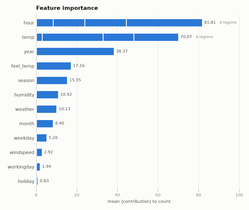
hour and temp have four curves each and the highest importance; the
trees at the bottom of the card are their regions. Why these two, and not
workingday or year, is the selection ledger:
calm.chain_.show()
  EXPLAINED VARIANCE
  ────────────────────────────────────────────────────────────────────────
    step         split on                 solo     ΔR²      R²       heter
    ──────────────────────────────────────────────────────────────────────
    GAM          (all features global)       —       —   65.8%           —
  + hour         temp, workingday, y…   +15.2%  +15.2%   81.1%     85 → 46
  + temp         hour, month             +2.8%   +1.6%   82.7%     33 → 23
    ──────────────────────────────────────────────────────────────────────
    FINAL                                                82.7%

  REJECTED SPLITS                                            min gain 1.0%
  ────────────────────────────────────────────────────────────────────────
    feature      split on                 solo     ΔR²    reason
    ──────────────────────────────────────────────────────────────────────
  ✗ year         hour                    +2.7%   -0.5%    redundant
  ✗ month        feel_temp, hour, hu…    +1.7%   +0.1%    below threshold
  ✗ workingday   hour                    +6.3%   -0.4%    redundant
  ✗ humidity     hour, season, temp      +1.9%   +0.5%    below threshold

    ✗ redundant: it would explain variance on its own (see solo),
      but the accepted splits already account for it.
Six features were candidates; two were split. workingday would explain
6.3% on its own, but hour is already conditioned on it, so its split is
redundant.
The curves
calm.plot_curves()
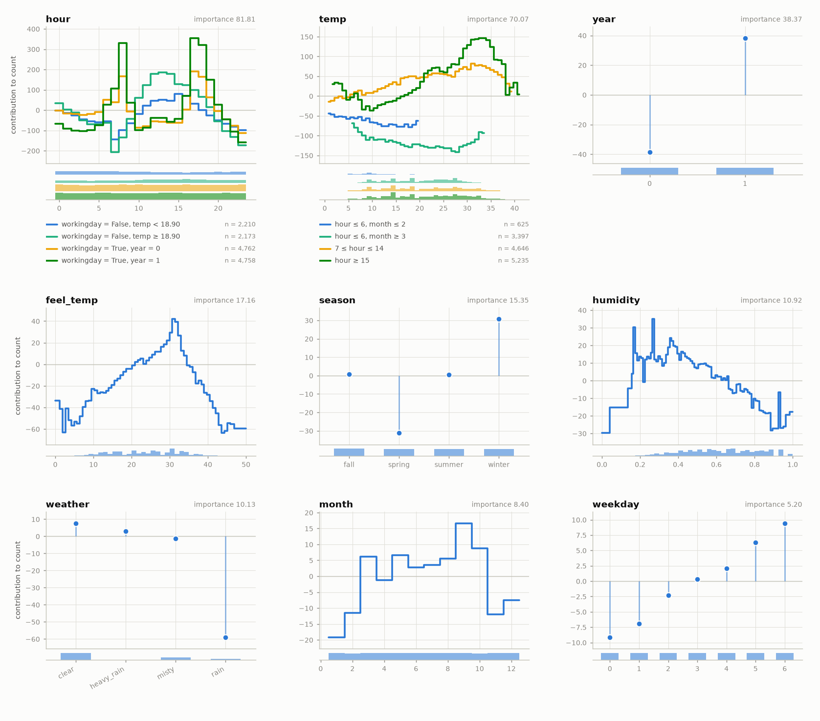
Panels are ordered by importance. Each curve is drawn only where its region
has data, and the strips under a panel show how the rows are spread, one row
of bars per region. Categorical features (season, weather, year) are
one mark per level.
calm.plot_curves("hour")
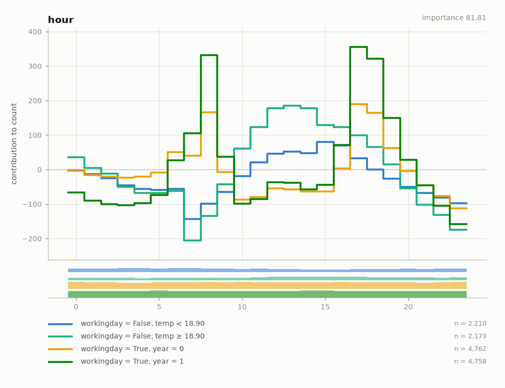
The hour panel shows what the GAM cannot: on working days rentals peak at
the commute hours, on days off they rise once around midday, and the
working-day shape is larger in the second year.
calm.plot_importance()
Why this prediction
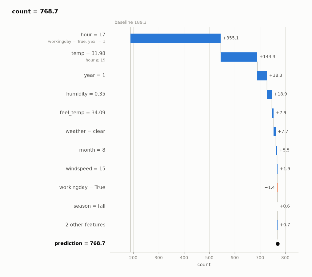
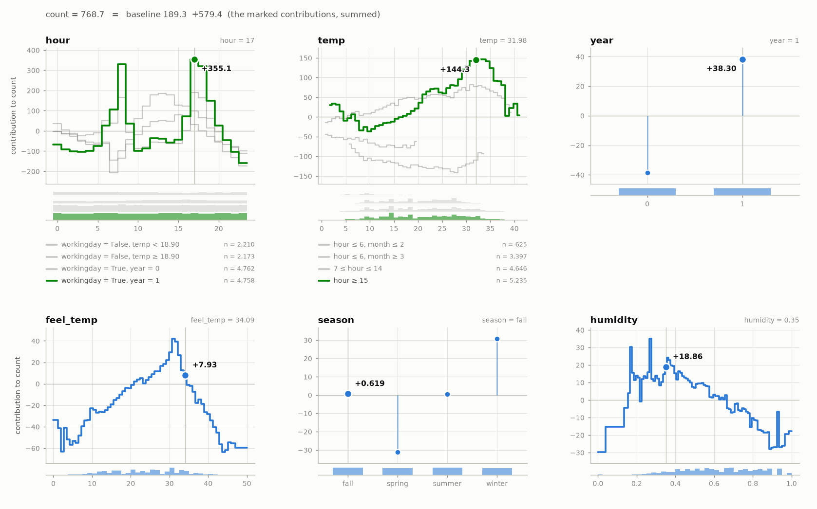
The held-out hour with the highest predicted count:
row = X_test.iloc[int(calm.predict(X_test).argmax())]
calm.print_prediction(row)
  PREDICTION                                                 count = 768.7
  ────────────────────────────────────────────────────────────────────────
    feature = value     because               contribution
    ──────────────────────────────────────────────────────────────────────
    hour = 17           workingday = True,          +355.1        │███████
                        year = 1
    temp = 31.98        hour ≥ 15                   +144.3        │███
    year = 1                                         +38.3        │█
    humidity = 0.35                                  +18.9        │
    feel_temp = 34.09                                 +7.9        │
    weather = clear                                   +7.7        │
    month = 8                                         +5.5        │
    windspeed = 15                                    +1.9        │
    workingday = True                                 −1.4        │
    season = fall                                     +0.6        │
    … 2 more features                                 +0.7        │
    ──────────────────────────────────────────────────────────────────────
    baseline (average prediction)                    189.3
    + contributions                                 +579.4
    = count                                          768.7
A working day of the second year at 5 pm, 32 °C: the commute peak of the
workingday = True, year = 1 curve adds 355 rentals to the average hour.
calm.plot_prediction(row)     # the same numbers as a waterfall
calm.plot_curves(at=row)      # the row marked on its curves
Where to next
- Choosing the knobs: try
max_partition_depth=1, or a highermin_r2_gain - How it works: where the regions come from
- API: estimators: everything
calmexposes afterfit