Aleatoric and epistemic uncertainty in classification problems
Discuss how categorical entropy can be used to quantify the aleatoric and epistemic uncertainty in Bayesian modeling.
Uncertainty Types
Machine Learning models may mispredict due to a variety of reasons. It is important to train models that know what they don’t know; to predict with uncertainty. Two specific types of uncertainty, aleatoric and epistemic, have attracted more attention since they cover two fundamental sources of mispredictions.
Aleatoric uncertainty describes the implicit variability of the data generating process, mainly due to unaccounted factors. Imagine we want to predict whether a student will pass or fail in the MSc degree from the following three attributes; the BSc grade $(x_1)$, the grade of the first MSc test $(x_2)$ and years passed from the BSc graduation $(x_3)$. With only these factors we are far from a perfect prediction. Numerous other attributes play an important role; his/her degree in each course of the BSc, his/her mental health, an unpredictable accident etc. All of them make the prediction feasible up to a specific level of (aleatoric) uncertainty.
Epistemic uncertainty describes our ignorance about a specific input; if we make a prediction for an input that is (very) different from the instances of the training set, we should also be uncertain. In the example above, lets say we want to evaluate a student with a high BSc grade that completely failed in the first MSc test, and, unfortunately, not many similar students (or none) exist at the training set. In supervised cases, as we move away from the examples of the training set, predictions are feasible up to a specific level of (epistemic) uncertainty.
The aleatoric $\mathcal{U}_a(x)$ and the epistemic $\mathcal{U}_e(x)$ component aggregate to express the uncertainty $\mathcal{U}$ of a prediction:
\[\mathcal{U}(x) = \mathcal{U}_a(x) + \mathcal{U}_e(x)\]Mathematical Formulation
Let’s quickly set up some notation. In this post, we cover the classification case, so we want to predict the correct class $c$ out of a set of $\mathcal{C}$. We fit a parametric model $f_{\theta}: \mathbf{x} \rightarrow y$ to the training set $\mathcal{D}$. We denote the parameter configuration that fits the data best with $\hat{\theta}$ $. The output $y = 1, 2, \ldots, |\mathcal{C}|$ is the index of the predicted class. For modeling the aleatoric and the epistemic uncertainty we need two extra ingredients.
For quantifying the aleatoric uncertainty, we need a trained model $\hat{\theta} $ that outputs a distribution $p(\mathbf{y}|\mathbf{x}, \hat{\theta} )$ over all possible classes, instead of only the winning class $y$. This means we need a probability vector $\mathbf{y}$, whose elements sum to $1$ and the $c$-th element $y_c$ is the probability of $c$, i.e., $p(y=c|\mathbf{x}, \hat{\theta} )$. For convenience, we also use $f_{\hat{\theta} }^c (\mathbf{x})$ to denote $y_c$. The probability vector $\mathbf{y}$ is the minimum requirement for quantifying the aleatoric uncertainty.
For quantifying the epistemic uncertainty, we need many models. Instead of a single model $\hat{\theta}$, we need the distribution over all parameters that describe the data well, i.e. the posterior distribution $p(\theta|\mathcal{D})$. Sometimes instead of accessing the PDF of the posterior, we need a way to sample from it: $\theta_k \sim p(\theta|\mathcal{D})$. We denote with $\tilde{\mathbf{y}}$ or $\tilde{p}(\mathbf{y}| \mathbf{x}, \mathcal{D})$ the expected prediction over the posterior distribution:
\[\tilde{\mathbf{y}} = \mathbb{E}_{ \theta | \mathcal{D} } [f_{\theta}(\mathbf{x})] \approx \frac{1}{K} f_{\theta_k}(\mathbf{x})\]Access to the posterior or a population of models is the minimum requirement for quantifying epistemic uncertainty.
Now that we know the requirements for modeling the aleatoric and the epistemic uncertainty, let’s see how entropy can be used to measure them.
Entropy
If we draw a sample $x_i$ from a discrete random variable $X$, the value $-\log p(x_i)$ quantifies our level of surprise or information gain. The level of surprise means how unexpected we considered the outcome. The information gain describes how much we learned after observing $x_i$. Imagine papers with written rules in a bowl. Player A draws a paper, reads the rules and designs how to offend. The other players design their defense without knowing what the paper writes. They only know that the bowl has $n_1$ papers with $\mathtt{rules_1}$, $n_2$ with $\mathtt{rules_2}$ etc. In other words, they know $p(x)$. If player A selects a rare paper, $p(x_i)$ is low, the information gain, $-\log p(x_i)$, is big because the other players have not prepared their defense for such an unexpected outcome, so player A has a big advantage. In the extreme, if the bowl contains only one set of rules, the gain is zero; the other players perfectly know what to expect.
I prefer the intuition behind the information gain because it helps me understand why to select $-\log p(x_i)$. For example, with the level of surprise, you may wonder why not simply use $1 - p(x_i)$, which maps the surprise into an intuitive linear scale of $[0, 1]$. In general, any function $f: [0,1] \rightarrow \mathbb{R}$ that is continuously decreasing in its domain could play this role. So, why choose $-\log$? The information gain dictates that if we observe two independent random variables, $x_i \sim X$ with information gain $H(x_i)$ and $y_i \sim Y$ with information gain $H(y_i)$, we want the total gain equal the sum. It is a meaningful property; if you learn $\alpha$ from a source and $\beta$ from another and the two pieces of information do not relate to each other, you have learned a total of $\alpha + \beta$. The logarithm family is the only one supporting $H(p(x_i, y_i)) = H(p(x_i)p(y_i)) = H(x_i) + H(y_i)$, so this is why $-\log$.
With this in mind, we can describe the entropy of a discrete distribution as the expected level of surprise or the expected information gain we will get after observing a sample:
\begin{equation} \mathbb{H}(p(x)) = \mathbb{E}_{X} [- \log p(x)] = - \sum p(x) \log p(x) \end{equation}
Entropy has its origins in Information Theory. For anyone interested, there are numerous excellent resources with interpretations about entropy
Entropy for Uncertainty
Here we focus on how entropy can be used to measure the uncertainty of a distribution. The concepts of surprise or information gain relate to uncertainty. The more uncertain, the more surprised I will get by the outcome or the bigger my information gain. Therefore, we can use entropy as a measure of the uncertainty of a discrete predictive distribution:
\begin{equation} \mathbb{H}( \mathbf{y}|\mathbf{x}, \theta) = - \sum_{c \in C} p(y_c|\mathbf{x}, \theta) \log p(y_c|\mathbf{x}, \theta) \end{equation}
Be careful with the log nature of entropy, it can be tricky. For example, in a binary classification problem, where the predictive distribution is $\mathbf{p} = (p_1, 1-p_1)$, the entropy as a function of $p_1$ is shown in the next figure.
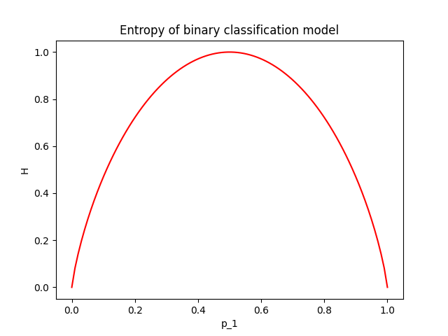
As we can see, entropy runs fastly in the beginning and slows down later. When the model predicts that the student will pass the MSc with $70\%$, we can instantly interpret that the prediction is 30% away from being certain. Another model that predicts $85\%$ pass can be directly compared to the first because we know what these extra $15$ percentage units are; they are 15 extra units of belief if you are a Bayesian and $15/100$ extra passes of the MSc if you are a Frequentist and you can repeat the experiment many times. \
Entropy makes such comparisons difficult due to the log scale. Entropy maps any discrete distribution to the range $[0, H_{max}]$. The maximum entropy is given when we allocate equal probability to all classes and depends on the number of classes; $H_{max} = log|\mathcal{C}|$. In the example above with maximum uncertainty equal to $H_{max} = log|\mathcal{C}|= 1$, the first prediction has $H_1=0.88$ and the second $H_2=0.61$. We know that the first prediction is more uncertain, but how much? We cannot (directly) interpret how much more certain the second model is.
Split into Aleatoric and Epistemic
Above, we considered a single model and used entropy to measure its uncertainty. In the Bayesian case, we have many models $\theta_k$ drawn from the posterior $p(\theta|\mathcal{D})$. We remind that the expected prediction is denoted with $\tilde{\mathbf{y}}$ and is computed as the mean prediction among the models, $ \tilde{\mathbf{y}} = \tilde{p}(\mathbf{y}| \mathbf{x}, \mathcal{D}) = \mathbb{E}_{\theta|\mathcal{D}} [f(\mathbf{x})] \approx \frac{1}{K} \sum_k f(\mathbf{x}) $. Entropy gives a convenient way to first compute the total uncertainty and then split it into the aleatoric and the epistemic component. The total uncertainty is the entropy of the expected prediction:
\[H(\mathbf{y} | \mathbf{x}, \mathcal{D}) = - \sum_{c \in \mathcal{C}} \tilde{p}(y_c | \mathbf{x}, \mathcal{D}) \log \tilde{p}(y_c | \mathbf{x}, \mathcal{D})\]The aleatoric component is the expected entropy over the entropy of each separate model $\mathbb{E}_{\theta|\mathcal{D}}[H(\mathbf{y}|\mathbf{x}, \theta)]$:
\[H_a(\mathbf{y} | \mathbf{x}, \mathcal{D}) = \mathbb{E}_{\theta|\mathcal{D}}[H(\mathbf{y}|\mathbf{x}, \theta)] \approx \frac{1}{K} \sum_k H(\mathbf{y}| \mathbf{x}, \theta_k)\]It is not obvious, but it always holds that $H(\mathbf{y} | \mathbf{x}, \mathcal{D}) > H_a(\mathbf{y} | \mathbf{x}, \mathcal{D})$. The epistemic component is the remainder, $H_e(\mathbf{y} | \mathbf{x}, \mathcal{D}) = H(\mathbf{y} | \mathbf{x}, \mathcal{D}) - H_a(\mathbf{y} | \mathbf{x}, \mathcal{D})$. And, finally, we reached the very convenient form:
\[H = H_a + H_e\]To get some intuition for the equations above, let’s see what happens in a simple binary classification example with two models sampled from the posterior. We freeze the expected prediction to $\mathbf{p} = (p_1, 1 - p_1)$, which is the average of model 1 with $\mathbf{p}^{(1)} = (p_1 - \Delta p, 1 - p_1 + \Delta p)$ and model 2 with $\mathbf{p}^{(2)} = (p_1 + \Delta p, 1 - p_1 - \Delta p)$. We change the value of $\Delta p$ to see how aleatoric and epistemic uncertainty behave.
Some intuition. Firstly, we expect that the total uncertainty remains constant; it is the entropy of the frozen expected prediction. We also expect that when $\Delta p = 0$, the two models perfectly match $\mathbf{p} = \mathbf{p}^{(1)} = \mathbf{p}^{(2)} = (p_1, 1 - p_1)$, so the epistemic component is zero and all the uncertainty comes from the aleatoric component. As $\Delta p$ increases, the aleatoric component (which is the mean entropy between the two models) lessens, giving space to the epistemic.
The figure below illustrates the evolution of the aleatoric and the epistemic components as $\Delta p$ grows, for $\mathbf{p} = (p_1=0.3, p_2=0.7)$.
The same evolution for an average prediction of $\mathbf{p} = (p_1=0.5, p_2=0.5)$.
And a table with numbers for $\mathbf{p} = (p_1=0.8, p_2=0.2)$.
| $\mathbf{p^{(1)}}$ | $H_1$ | $\mathbf{p^{(2)}}$ | $H_2$ | $\mathbf{p}$ | $H$ | $H_a$ | $H_e$ |
|---|---|---|---|---|---|---|---|
| $(0.8, 0.2)$ | $0.72$ | $(0.8, 0.2)$ | $0.72$ | $(0.8, 0.2)$ | $0.72$ | $0.72 \; (100\%)$ | $0 \; (0\%)$ |
| $(0.85, 0.15)$ | $0.61$ | $(0.75, 0.15)$ | $0.81$ | $(0.8, 0.2)$ | $0.72$ | $0.71 \; (98.43\%)$ | $0.01 \; (1.57\%)$ |
| $(0.9, 0.1)$ | $0.47$ | $(0.7, 0.3)$ | $0.88$ | $(0.8, 0.2)$ | $0.72$ | $0.68 \; (93.52\%)$ | $0.05 \; (6.48\%)$ |
| $(0.95, 0.05)$ | $0.29$ | $(0.65, 0.35)$ | $0.93$ | $(0.8, 0.2)$ | $0.72$ | $0.61 \; (84.53\%)$ | $0.11 \; (15.47\%)$ |
| $(1, 0)$ | $0$ | $(0.6, 0.4)$ | $0.97$ | $(0.8, 0.2)$ | $0.72$ | $0.49 \; (67.2\%)$ | $0.24 \; (32.75\%)$ |
We observe that due to the log nature of entropy, it is difficult to interpret aleatoric and epistemic uncertainties as absolute values or as percentages of the total uncertainty. If somebody tells you that the total uncertainty in a binary classification problem is $H = 0.72$, you don’t exactly understand how uncertain the final prediction is, even though you can compute that in binary problems $H_{max} = \log|\mathcal{C}| = 1$. If (s)he continues, that out of $H=0.72$, the aleatoric uncertainty is $H_a=0.61$ ($84.53\%$ of $H$) and the epistemic $H_e=0.11$ ($15.47\%$ of $H$), you can understand that models agree ($H_e$ is small) and most of the uncertainty is because of the aleatoric component. All these would be much clearer if you simply inspect the individual model predictions, $p^{(1)} = (0.95, 0.05)$ and $p^{(2)} = (0.65, 0.35)$. You could then understand that even though they both vote for option 1, they significantly disagree on how certain they are, information that is not that clear by just viewing $H_e = 15.47\%$ of $H$. But, inspecting all different model predictions one by one is not easy if you have many models or the whole posterior distribution. In these cases, entropy provides a convenient summary statistic that respects $H = H_e + H_a$.
Conclusion
Entropy maps any categorical distribution to three summary statistics; the aleatoric $H_a$, the epistemic $H_e$ and the total uncertainty $H = H_a + H_e$. It simply requires samples from the posterior distribution $\theta_k \sim p(\theta | \mathcal{D})$ and access to the model $f_\theta(\mathbf{x})$.
The range of uncertainties is $[0, H_{max}]$; $H = 0$ means no-uncertainty, $H = H_{max}$
Choosing whether to trust the prediction, can be easily decided based on the epistemic entropy. Check the following table:
| $H_a$ | $H_e$ | Take-away | Interpretation |
|---|---|---|---|
| low | low | Trust the certain prediction | Models agree on a certain prediction |
| high | low | Trust the uncertain prediction | Model aggree that they can predict with some uncertainty. |
| low | high | Don’t trust the prediction | The input is away from the training data manifold. |
| high | high | Don’t trust the prediction | The input is away from the training data manifold. |
If $H_e$ is small, models agree so we can trust their outcome; if they are all certain, we can follow the prediction if they are all uncertain, we know that we are on an edge case where the features do not provide enough information to separate the classes. If $H_e$ is big, you cannot trust the prediction, because the models have not seen similar inputs on the training set.
Disadvantages
The table above is very helpful. But what is low and what is high? It is difficult to provide a specific number. For binary problems, if $0 \leq H \leq 0.2 * H_{max}$, the prediction is very certain (close to $95\% - 5\%$). Unfortunately, It is even more difficult to define a threshold for a high or a low epistemic entropy. For these reasons, even though $H_e$ and $H_a$ are helpful for a quick interpretation, we need to check more summary statistics for a detailed understanding of the uncertainty of a Bayesian prediction.